Analyzing high-dimensional data with {rrda}
a_analyzing_high_dim_omics_data.RmdThis vignette illustrates the use of the rrda package,
dedicated to ridge redundancy analysis for high-dimensional omics
data.
While conventional methods of RDA (or RRDA) are restricted to relatively small matrices, rrda extends these computations to high-dimensional data—including datasets with more than 100,000 features.
This capability makes it especially valuable in modern omics sciences and other fields where analyzing extremely large datasets is essential.
Requirements
The packages required for the analysis are `rrda`` plus some others for data manipulation and representation:
Mathematical background
Classic formula
The Ridge Redundancy Analysis model is represented as:
Let be an matrix of response variables, and let be an matrix of predictor variables. We assume that the columns of matrices and are centered to have means of 0.
The relation between and is given by
where is the matrix of regression coefficients, and is an error matrix.
The ridge RDA aims to estimate under both rank and ridge restrictions. The corresponding optimization problem is
where is the Frobenius norm and is the ridge regularization parameter.
For High-Dimensional Data
For Ridge Redundancy Analysis, the ridge estimator can be decomposed as follows:
where the Singular Value Decomposition (SVD) of is and are the SVD components of
Since
depends on
,
its SVD must be computed for each value of
.
However, efficiency can be gained because
is the product of:
- a diagonal matrix
,
and
- a constant matrix (independent of ).
Simulation
Parameter tuning
cv_result <- rrda.cv(Y = Y, X = X, nfold = 5)
#> Call:
#> rrda.cv(Y = Y, X = X, lambda = 4.801 - 48010, maxrank = 15, nfold = 5)
rrda.summary(cv_result = cv_result)
#> === opt_min ===
#> MSE:
#> [1] 1.218769
#> rank:
#> [1] 5
#> lambda:
#> [1] 66.71
#>
#> === opt_lambda.1se ===
#> MSE:
#> [1] 1.244403
#> rank:
#> [1] 5
#> lambda:
#> [1] 248.7
#>
#> === opt_rank.1se ===
#> MSE:
#> [1] 1.218769
#> rank:
#> [1] 5
#> lambda:
#> [1] 66.71
Visualize Results
Here we illustrate the parameter tuning process (regularization path), which helps identify the optimal parameter for maximizing prediction accuracy from X to Y.
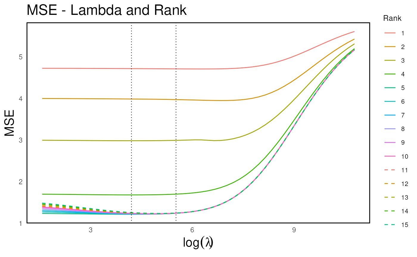
h <- rrda.heatmap(cv_result) # cv result heatmap
print(h)
best_lambda <- cv_result$opt_min$lambda  # selected parameter
best_rank <- cv_result$opt_min$rank # selected parameter

Bhat <- rrda.fit(Y = Y, X = X, nrank = best_rank, lambda = best_lambda) # fitting
Bhat_mat <- rrda.coef(Bhat)
#> rank:
#> [1] 5
#> lambda:
#> [1] 66.71
Yhat_mat <- rrda.predict(Bhat = Bhat, X = X) # prediction
Yhat <- Yhat_mat[[1]][[1]][[1]] # predicted values

cor_Y_Yhat <- diag(cor(Y,Yhat)) # correlation
summary(cor_Y_Yhat)
#>    Min. 1st Qu.  Median    Mean 3rd Qu.    Max.
#>  0.4813  0.8754  0.9131  0.8964  0.9371  0.9813

plot(Y, Yhat)
abline(0, 1, col = "red")
title(sub = "Fitted values vs observations")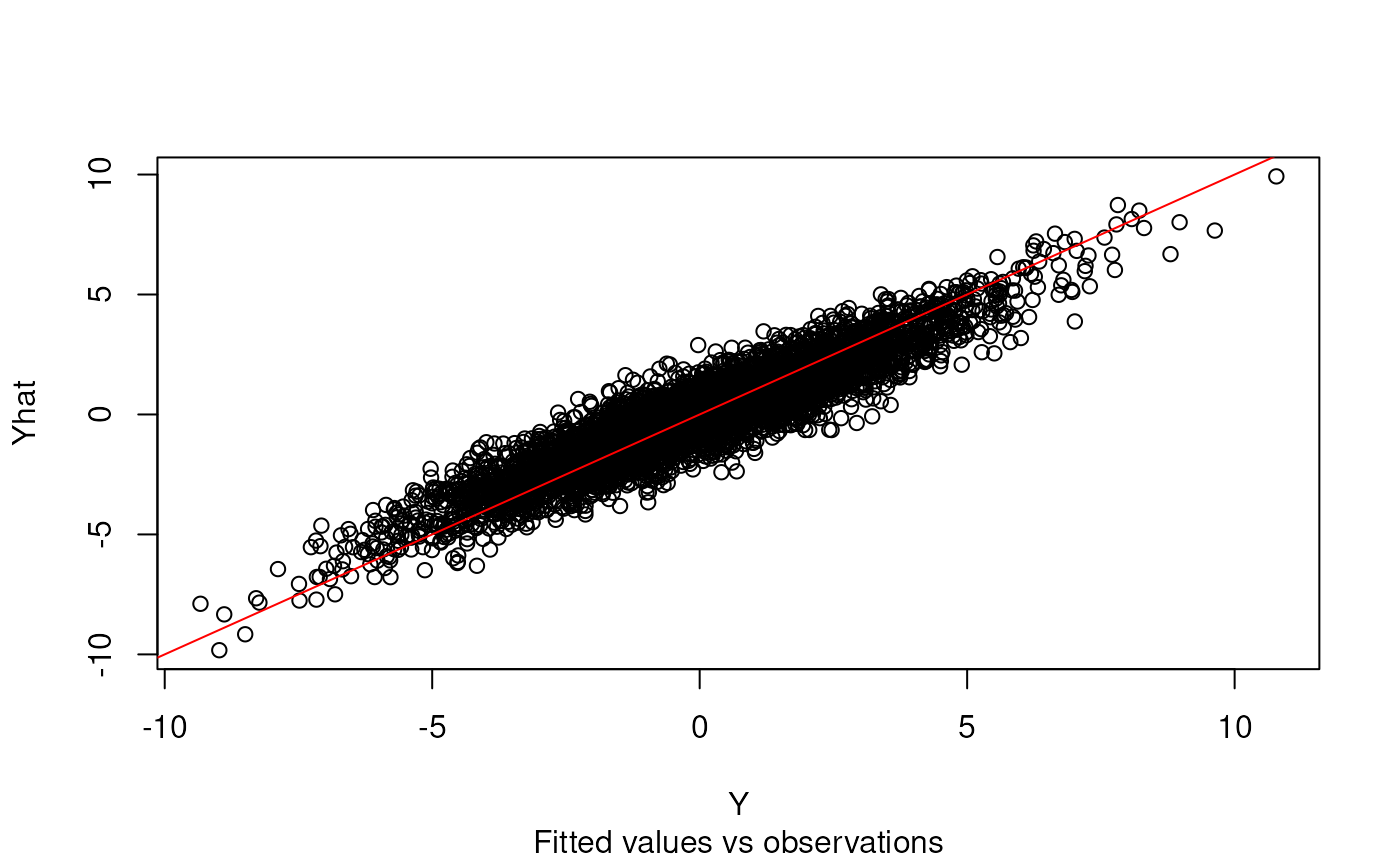
Two-Dimensional Plot
Traditionally, (Ridge) RDA is visualized in two
dimensions.
However, in omics studies, this approach can sometimes overload
the plot with information, making interpretation
challenging.
# You want to specify one lambda in `rrda.fit` to visualize

ud <- Bhat$Bhat_comp[[1]][[1]] # SVD component of B (UD)
v <- Bhat$Bhat_comp[[1]][[2]] # SVD component of B (V)

ud12 <- ud[, 1:2]
v12 <- v[, 1:2]

# Base plot: ud (e.g., site scores)
plot(v12,
     xlab = "RRDA1", ylab = "RRDA2",
     xlim = range(c(ud12[,1], v12[,1])) * 1.1,
     ylim = range(c(ud12[,2], v12[,2])) * 1.1,
     pch = 19, col = "darkgreen",
     main = "RRDA")

# Add v (e.g., species scores) as arrows from origin
arrows(0, 0, ud12[,1], ud12[,2], col = "blue3", length = 0.1)

# Optionally add text labels
text(ud12, labels = paste0("X", 1:nrow(ud12)), pos = 3, col = "blue3", cex = 0.6)
text(v12, labels = paste0("Y", 1:nrow(v12)), pos = 3, col = "darkgreen", cex = 0.6)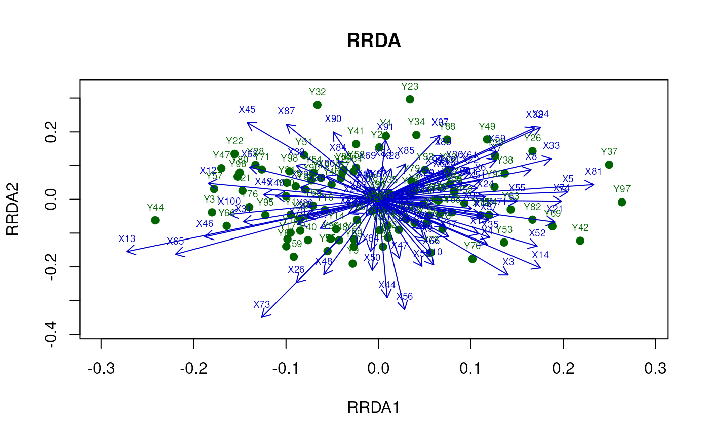
Top Feature Heatmap
For better interpretability, we visualize the feature–feature matrix using a selected dimensionality, highlighting the most informative features.
best_lambda <- cv_result$opt_min$lambda
best_rank <- cv_result$opt_min$rank
rrda.top(Y = Y, X = X, nrank = best_rank, lambda = best_lambda, mx = 20, my = 20)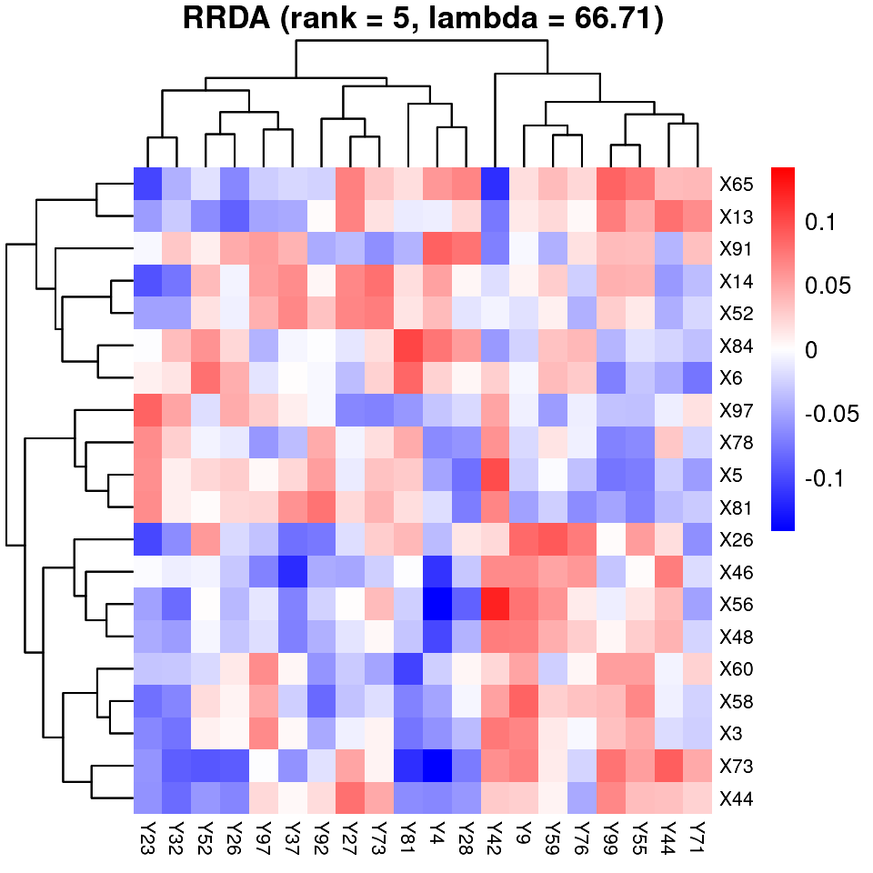
References
Yoshioka H, Aubert J, Mary-Huard T (????). rrda: Ridge Redundancy Analysis for High-Dimensional Omics Data. R package version 0.2.3, https://cran.r-project.org/package=rrda
Yoshioka, H., Aubert, J., Iwata, H., and Mary-Huard, T., 2025. Ridge Redundancy Analysis for High-Dimensional Omics Data. bioRxiv, doi: 10.1101/2025.04.16.649138
@article {Yoshioka2025.04.16.649138,
    author = {Yoshioka, Hayato and Aubert, Julie and Iwata, Hiroyoshi and Mary-Huard, Tristan},
    title = {Ridge Redundancy Analysis for High-Dimensional Omics Data},
    elocation-id = {2025.04.16.649138},
    year = {2025},
    doi = {10.1101/2025.04.16.649138},
    URL = {https://www.biorxiv.org/content/early/2025/09/10/2025.04.16.649138},
    eprint = {https://www.biorxiv.org/content/early/2025/09/10/2025.04.16.649138.full.pdf},
    journal = {bioRxiv}
}